Now that we’ve dealt with the direct material and direct labour parts of production, what about looking at overheads? Of course, we have variance calculations for overheads as well. We even split it up between fixed and variable overheads.

Let’s now make it more challenging and do both fixed and variable overheads in the same calculation with a more complex example.

Example information:
Budgeted production output was 600 units. Budgeted variable overheads were £900. Budgeted fixed overheads were £480. Overheads are absorbed according to machine hours. Machine hours were budgeted at 0.50 hours per unit. Actual production output was 580 units, actual variable overheads were £825, actual fixed overheads were £520, total machine hours were 270.

Step 1 – Since it is not given, we need to calculate what the standard absorption rates are for fixed and variable overheads. We first take the budgeted production output and multiply it by the machine hours per unit = 600 units x 0.50 hours = 300 total budgeted machine hours.

Step 2 – We then take the budgeted variable overheads and divide it by the total budgeted machine hours = £900 / 300 = £3.00 is the variable overhead absorption rate. We will do the same for the budgeted fixed overheads and divide it by the total budgeted machine hours = £480 / 300 = £1.60  is the fixed overhead absorption rate.

Step 3 – We then take budgeted machine hours per unit and multiply it with the rates. For variable overhead rate, it is 0.50 hours x £3.00 = £1.50. For fixed overhead rate, it is 0.50 hours x £1.60 = £0.80. These are the standard rates/costs.

Step 4 – Now let’s do actuals! To calculate the expenditure variances, we will need to know the actual overheads figures and we will need to use the actual machine hours spent and multiply it with the absorption rates.

Actual variable overheads = £825
Actual quantity (number of machine hours) is 270 hours and multiply this with the variable overheads absorption rate of £3.00 = £810
The difference of £825 – £810 = £15 is the variable overheads expenditure variance and is an adverse one in this case.

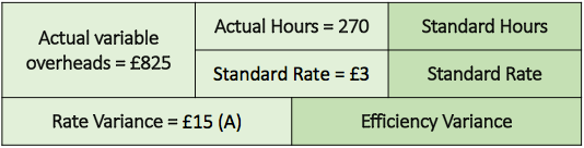
Note that I will now start denoting an adverse variance with an (A) after the figure, and a favourable variance will have an (F) after the number.

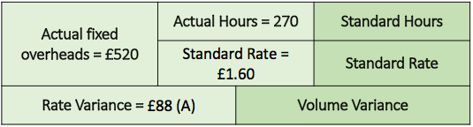
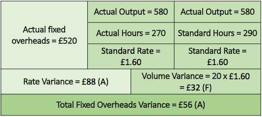
Actual fixed overheads = £520
Actual quantity (number of machine hours) is 270 hours and multiply this with the fixed overheads absorption rate of £1.60 = £432
The difference of £520 – £432 = £88 is the fixed overheads expenditure variance and like above variance, is an adverse one as well.

Step 5 – To calculate the volume and efficiency variances, we will need to alter the way we look at the information a little bit. For some students, it can be an easy switch in outlook, but for others, it can leave you scratching your heads. So I’ll try and make it practical.

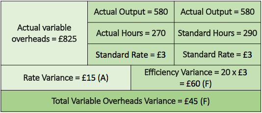
For efficiency, we should be looking at how much hours did we spend producing vs how much hours it should have been. Have a look at below calculation:

Actual output is 580, which took 270 actual hours to produce. As per budget, each unit should have taken 0.50 hours to make. If we take the actual output and multiply it with the budgeted machine hour per unit (580 x 0.50), it should have taken us 290 hours. But instead, we only took 270 hours. This is a favourable difference because it has taken us faster to produce more output. We are more efficient!

To value this efficiency difference, we will need to take the differences in hours (290 – 270 = 20) and multiply this with the variable overhead absorption rate of £3.00 to place a value (20 x £3.00). The difference of £60.00 is a favourable variable overheads efficiency variance.

Let’s go a bit further and calculate total variable overheads variance. I probably should point out that having an adverse variance on one side and favourable variance on the other would matter in the total calculation. Adverse and favourable variances have the opposite effect on each other. So if you ever encounter this scenario (as we have above), we would need to calculate the difference rather than the sum of the rate and efficiency variances.

For volume, we should be looking at how much we produced (quantity of units) vs how much was budgeted for.

To calculate the fixed overheads volume variance, we should find the difference between the budgeted output of 600 units and actual units of 580. This particular difference is an adverse one since we have produced less than what was planned (600 – 580 = 20). To place a value, we should take this difference and multiply it with the fixed overheads standard rate of £1.60 to get the result of £32.00 (20 x £1.60).

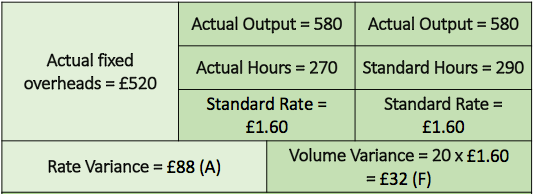
And for the total fixed overheads variance:

Shall we stop here? There are more sets that I’d like to cover the next few weeks – planning, mix and yield variances. Whoever thought that there would be so much variance analyses? I certainly did. Didn’t I say that when I first started this series?

Operational OT course available here.