So if I haven’t made you run away with Part 1, then I must have done something right. Welcome to Part 2 of Variance Analysis.

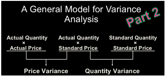
Remember our memorised visual two weeks ago? If you’ve got it stuck in your mind, then that’s good. That’s how we wanted it all along. For those who’ve forgotten, here it is again.

We made use of this table for a couple of variances. This week, we will look at direct labour and overheads variances. The concept is not different from how we worked out direct material variances. Only the terms change with regards to whether it is a price variance, usage variance, efficiency variance, volume variance, expenditure variance, etc. But I’m getting way ahead of you guys.

Let me start by introducing 2 direct labour variance – direct labour rate variance and direct labour efficiency variance.

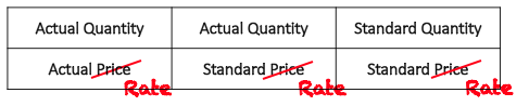
In this instance, because we are dealing with rates, scratch out the price on the table and call it rate for a second, like so.

So now let’s start with our variances and take direct labour rate variance. Similar to how we did our calculations when dealing with direct material, the same goes for direct labour. We never like overcomplicating things so we tweak the same example information with just slight changes to the numbers. We will also note that the quantity is now based according to how many hours and the rate is the labour rate per hour.

Example information: Actual value of production hours was £7000. Actual number of production hours was 1000 hours. It was originally forecast at £5 per hour.

So we will do the calculations as follows:
Actual value at actual rate = £7000 (we can easily calculate this out since we know the actual production hours, and if we do, we work out that actual rate used was £7000/1000 hours = £7)
Actual production hours = 1000 x standard rate at £5 = £5000

The difference of £2000 is a rate difference (because we are calculating the difference between rate rather than quantity or number of actual hours). And since actual rate is much higher than the standard rate, this direct labour rate variance is an adverse one.

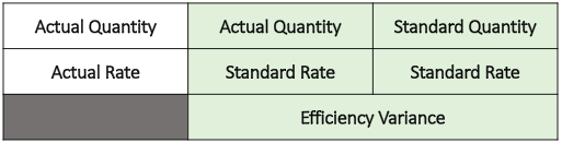
Looking at above table, what happens to Columns 2 and 3? The difference between these 2 columns affect the actual and standard quantity (number of spent hours) and so will generate the direct labour efficiency variance.

Example information: Actual number of production hours spent was 1000. It was originally budgeted to spend 1200 at a rate of £5 per hour.

The calculations would be as follows:
Actual number of production hours = 1000 x standard rate at £5 = £5000
Standard number of production hours = 1200 x standard rate at £5 = £6000

The direct labour efficiency variance of £1000 arises from producing the goods in less time than originally budgeted for and so this variance is considered to be a favourable one.

The sum of direct labour rate variance and direct labour efficiency variance is the total direct labour variance. In this calculation, the total direct labour variance is then calculated as (Adverse) £2000 + (Favourable) £1000 = (Adverse) £1000.

To check:
Actual value at actual rate = £7000
Standard number of production hours = 1200 x standard rate at £5 = £6000
The difference is £7000 – £6000 = £1000 adverse, which confirms above result.

The next segment of variance analysis will be a  longer one dealing with overheads and so I’m going to end this one off here for now. Tune in next week for our third instalment.

P.S. If you’d like to get your hands on the P1 study text, why not visit Astranti to have a look at what they have on offer?